Recovering the 1D material properties

Generating the mesh

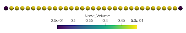
The file input_mesh.yaml in the example folder will generate the mesh as shown in the following figure.

Setup the simulation

The file input.yaml in the example folder contains following code snippets to setup the simulation.

Model

The quasi-static models as described in [1] is used to assemble the tangent stiffness matrix and obtain the solution by solving Newton steps.

Model:
  Dimension: 1
  Discretization_Type:
    Spatial: finite_difference
    Time: quasi_static
  Final_Time: 1
  Time_Steps: 1
  Horizon: 1
  Horizon_h_Ratio: 3
Mesh:
  File: mesh.vtu

Material model

The state-based elastic material models as described in [2] is implemented for the ElasticState material.

Material:
  Type: ElasticState
  Density: 1
  Compute_From_Classical: true
  E: 4000
  Influence_Function:
    Type: 1

Applying boundary conditions

Displacement boundary conditions

The following code applies a fixed displacement to the first node on the left-hand side in the first figure.

Displacement_BC:
  Sets: 1
  Set_1:
    Location:
      Line: [-0.1, 0.3]
    Direction: [1]
    Time_Function:
      Type: constant
      Parameters:
        - 0.0
    Spatial_Function:
      Type: constant

Force boundary conditions

The following code applies a external body force density to the last node on the right-hand side in the first figure. Note that in this example we want to apply a force $F=40$, however since the last node has a volume $v=0.25$ this results in a body force density $b=40/0.25=166$.

Force_BC:
  Sets: 1
  Set_1:
    Location:
      Line: [15.9, 16.5]
    Direction: [1]
    Time_Function:
      Type: linear
      Parameters:
        - 1
    Spatial_Function:
      Type: constant
      Parameters:
        - 160

Solver

Solver:
  Type: ConjugateGradient
  Max_Iteration: 1000
  Tolerance: 1e-9
  Perturbation: 1e-7

Validation

Forces

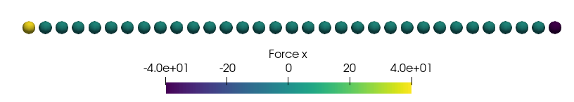
All the forces in the mid of the bar are zero, except the forces at the boundary which are $F=40$ on the right-hand side and $F=-40$ on the left-hand side. This corresponds to the loading we applied.

Stress

The stress in classical continuum mechanics is given as $\sigma=F/S$, where $F$ is the applied force and $S$ is the surface area of the bar. Assuming a surface area $S=1$ leads to $\sigma=40/1=40$ which matches the stress in the Figures for the nodes in the center of the bar. Note that the nodes close to the boundary have non-matching values due to the so-called surface effect.

Strain

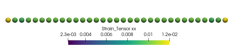
The strain in classical continuum mechanics is given as $\epsilon=F/(S\cdot E)=40/(1\cdot 4000)=0.01$ which matches for the nodes in the center of the bar. Note that the nodes close to the boundary have non-matching values due to the so-called surface effect.

Strain energy

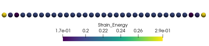
The strain energy in classical continuum mechanics is given as $U=\sigma^2/(2\cdot E)=40^2/(2\cdot 4000)=0.2$ which matches for the nodes in the center of the bar. Note that the nodes close to the boundary have non-matching values due to the so-called surface effect.

References

1. Littlewood, David J. “Roadmap for peridynamic software implementation.” SAND Report, Sandia National Laboratories, Albuquerque, NM and Livermore, CA (2015).
2. Silling, Stewart A., et al. “Peridynamic states and constitutive modeling.” Journal of Elasticity 88.2 (2007): 151-184.